Plot SpatialRD output

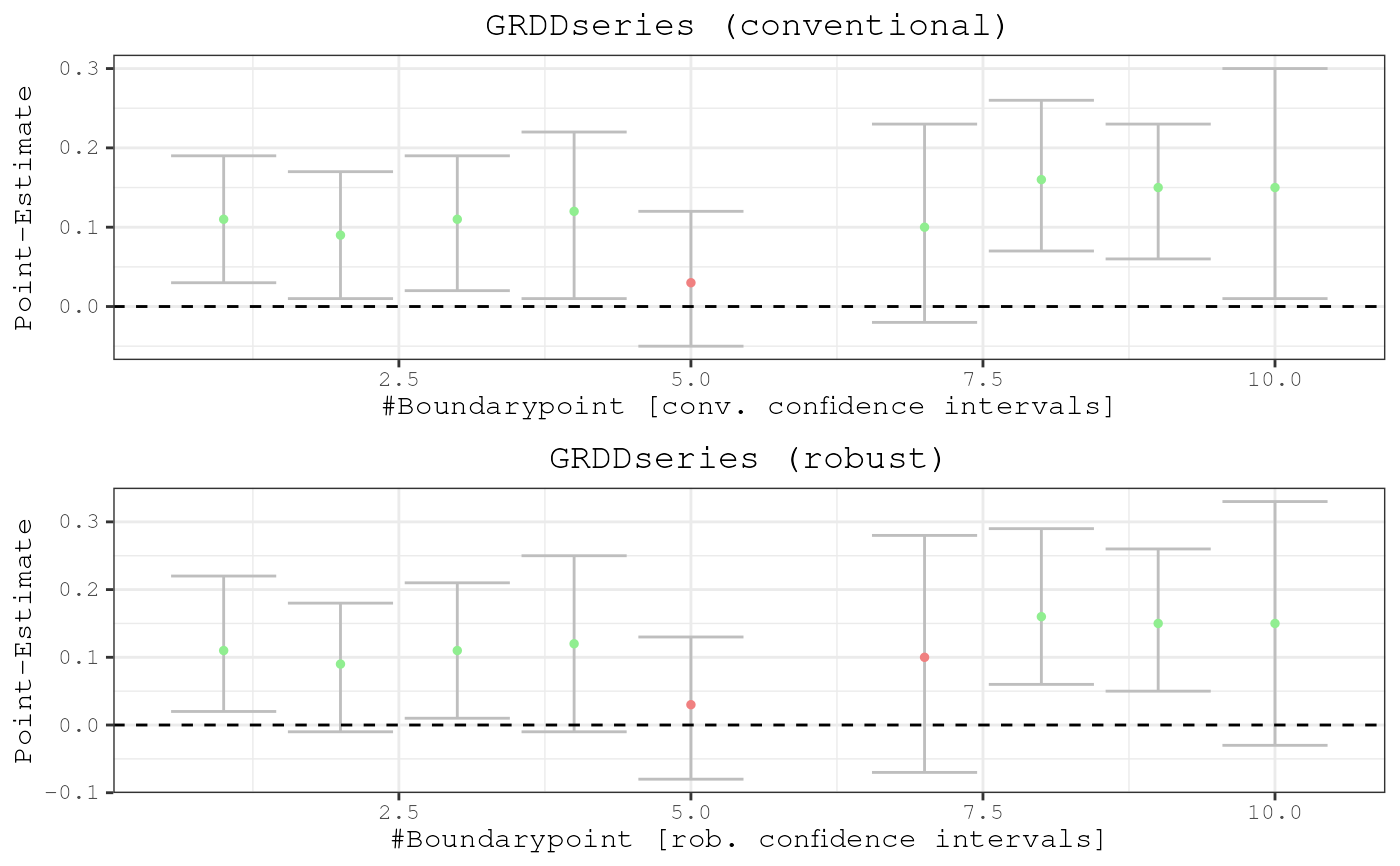
Produces plot of GRDDseries and optionally of a map that visualises every point estimate in space.

plotspatialrd(SpatialRDoutput, map = FALSE)

Arguments

SpatialRDoutput

spatial object that is produced by an estimation with spatialrd

map

TRUE/FALSE depending on whether mapplot is desired (make sure to set spatial.objcet = TRUE in the spatialrd function)

Value

plots produced with ggplot2

Examples

points_samp.sf <- sf::st_sample(polygon_full, 1000) # create points
# make it an sf object bc st_sample only created the geometry list-column (sfc):
points_samp.sf <- sf::st_sf(points_samp.sf)
# add a unique ID to each observation:
points_samp.sf$id <- 1:nrow(points_samp.sf)
# assign treatment:
points_samp.sf$treated <- assign_treated(points_samp.sf, polygon_treated, id = "id")
#> Warning: attribute variables are assumed to be spatially constant throughout all geometries
# first we define a variable for the number of "treated" and control
NTr <- length(points_samp.sf$id[points_samp.sf$treated == 1])
NCo <- length(points_samp.sf$id[points_samp.sf$treated == 0])
# the treated areas get a 10 percentage point higher literacy rate
points_samp.sf$education[points_samp.sf$treated == 1] <- 0.7
points_samp.sf$education[points_samp.sf$treated == 0] <- 0.6
# and we add some noise, otherwise we would obtain regression coeffictions with no standard errors
points_samp.sf$education[points_samp.sf$treated == 1] <- rnorm(NTr, mean = 0, sd = .1) +
  points_samp.sf$education[points_samp.sf$treated == 1]
points_samp.sf$education[points_samp.sf$treated == 0] <- rnorm(NCo, mean = 0, sd = .1) +
  points_samp.sf$education[points_samp.sf$treated == 0]

# create distance to cutoff
points_samp.sf$dist2cutoff <- as.numeric(sf::st_distance(points_samp.sf, cut_off))

points_samp.sf$distrunning <- points_samp.sf$dist2cutoff
# give the non-treated one's a negative score
points_samp.sf$distrunning[points_samp.sf$treated == 0] <- -1 *
 points_samp.sf$distrunning[points_samp.sf$treated == 0]

# create borderpoints
borderpoints.sf <- discretise_border(cutoff = cut_off, n = 10)
borderpoints.sf$id <- 1:nrow(borderpoints.sf)

# finally, carry out estimation alongside the boundary:
results <- spatialrd(y = "education", data = points_samp.sf, cutoff.points = borderpoints.sf,
treated = "treated", minobs = 20, spatial.object = FALSE)


plotspatialrd(results)