SpatialRDD: get started

In recent years, spatial versions of Regression Discontinuity Designs (RDDs) have increased tremendously in popularity in the social sciences. In practice, executing spatial RDDs, especially the many required robustness- and sensitivity checks, is quite cumbersome. It requires knowledge of statistical programming and handling and working with geographic objects (points, lines, polygons). Practitioners typically carry out these GIS tasks in a “point and click” fashion in GUIs like ArcGIS, QGIS, or GeoDA and then manually export these data into the statistical environment of their choice. Statistical analysis is then carry out in an a-spatial way. This is sub-optimal for several reasons:

it is very time consuming and cumbersome
it is prone to errors
it is not reproducible
it is not very flexible and makes it harder to understand the data at hand

SpatialRDD is the first (geo-)statistical package that unifies the geographic tasks needed for spatial RDDs with all potential parametric and non-parametric estimation techniques that have been put forward (see e.g. Lehner2023a? for an overview). It makes it easy to understand critical assumptions regarding bandwidths, sparse border points, and border segment fixed effects. Furthermore, the flexibility of the shift_border function makes it attractive for all sorts of identification strategies outside of the RD literature that rely on shifting placebo borders.

Geographic objects are treated as simple features throughout, making heavy use of the sf package by Edzer Pebesma which revolutionized spatial data analysis in R and has already superseded the older and less versatile sp package.
SpatialRDD facilitates analysis inter alia because it contains all necessary functions to automatize otherwise very tedious tasks that are typically carried out “by hand” in the GUIs of GIS software. SpatialRDD unifies everything in one language and e.g. has the necessary functions to check and visualize the implications of different bandwidths, shift placebo boundaries, do all necessary distance calculations, assign treated/non-treated indicators, and flexibly assign border segment fixed effects while keeping the units of observations at their proper position in space and allowing the researcher to visualize every intermediate step with map plots. For the latter we will mostly rely on the flexible and computationally very efficient tmap package, while also ggplot2 is used at times.
For the purpose of illustration, this vignette uses simulated data on real boundaries/polygons and guides the user through every necessary step in order to carry out a spatial RDD estimation. At the appropriate points, we will also make remarks on technical caveats and issues that have been pointed out in the literature and give suggestions to improve these designs.
The workhorse functions of SpatialRDD in a nutshell are:

and they are going to be introduced here in precisely this order.

Some words of caution

You (obviously) have to pay attention that you have an RD border that is fine-grained enough so that it resembles the true cutoff. Something at the degree of e.g. the widely used GADM boundaries (just as an example, because administrative boundaries themselves are usually never valid RD cutoffs due to the compound treatment problem) is most probably not detailed enough. Furthermore, I suggest to transform your data into a projected CRS and work on the euclidean plane (instead of on the sphere with angles, that is, with longitude and latitude). A good choice would be UTM: find the right grid here, then get the corresponding EPSG number and use it in st_transform() after you imported your data (see e.g. Bivand and Pebesma 2023 for guidance on projection systems).

Setup and Propaedeutics

Throughout the vignette we will use the geographic boundaries on Goa, India, from Lehner (2023). The data, included in the package, contains

a line called cut_off which describes the spatial discontinuity
a polygon that defines the “treated” area
a polygon that defines the full study area (which is going to be useful as this defines the bounding box)

For your own RD design you need 1. in the form of either a line (as a single feature, i.e. all potential segments merged together) or a finely spaced set of points on your border. Furthermore you need the polygon that specifies the treatment area, and, of course, the data set that contains all your observations, including the x- and y-coordinate for each unit of observation. This way it is easy to convert the data to an sf data.frame.

library(SpatialRDD)
library(dplyr) # more intuitive data wrangling
library(stargazer) # easy way to make model output look more appealing (R-inline, html, or latex)
library(sf)

The data shown here come in EPSG:32643, which is a “localized” UTM projected coordinate reference system (CRS). If your study area is small, you should consider reprojecting your data into the CRS of the according UTM zone (simply use st_transform()) - or choose a different projection in case it is more appropriate to your study area. To verify the units of our CRS we could simply run st_crs(cut_off)$units.

All the spatial objects are of class sf from the sf package. This means they are just a data.frame with a special column that contains a geometry for each row. The big advantage is, no matter if you prefer base R, dplyr, or any other way to handle and wrangle your data, the sf object can be treated just like a standard data.frame. The one single step that transforms these spatial objects back to a standard data.frame is just dropping the geometry column with

st_geometry(any.sf.object) <- NULL

or alternatively

st_set_geometry(any.sf.object, NULL)

If you import geospatial data in a different format, say the common shapefile (*.shp) - which is NOT preferrable see here why, or as a geopackage (*.gpkg), it is fairly straightforward to convert it:

mydata.sf <- st_read("path/to/file.shp")

In case your data is saved as a *.csv (if in Stata file format, check the foreign and readstata13 package) you just have to tell sf in which columns the x- and x-coordinates are saved, and it will convert it into a spatial object:

mydata.sf <- st_as_sf(loaded_file, coords = c("longitude", "latitude"), crs = projcrs) 
# just the EPSG as an integer or a proj4string of the desired CRS

For more thorough information, I suggest consulting the documentation and vignettes of the sf package or Bivand and Pebesma (2023).

Inspecting the Study Area & simulating Data

data(cut_off, polygon_full, polygon_treated)
library(tmap)
#> Breaking News: tmap 3.x is retiring. Please test v4, e.g. with
#> remotes::install_github('r-tmap/tmap')
tm_shape(polygon_full) + tm_polygons() + 
  tm_shape(polygon_treated) + tm_polygons(col = "grey") + 
  tm_shape(cut_off) + tm_lines(col = "red")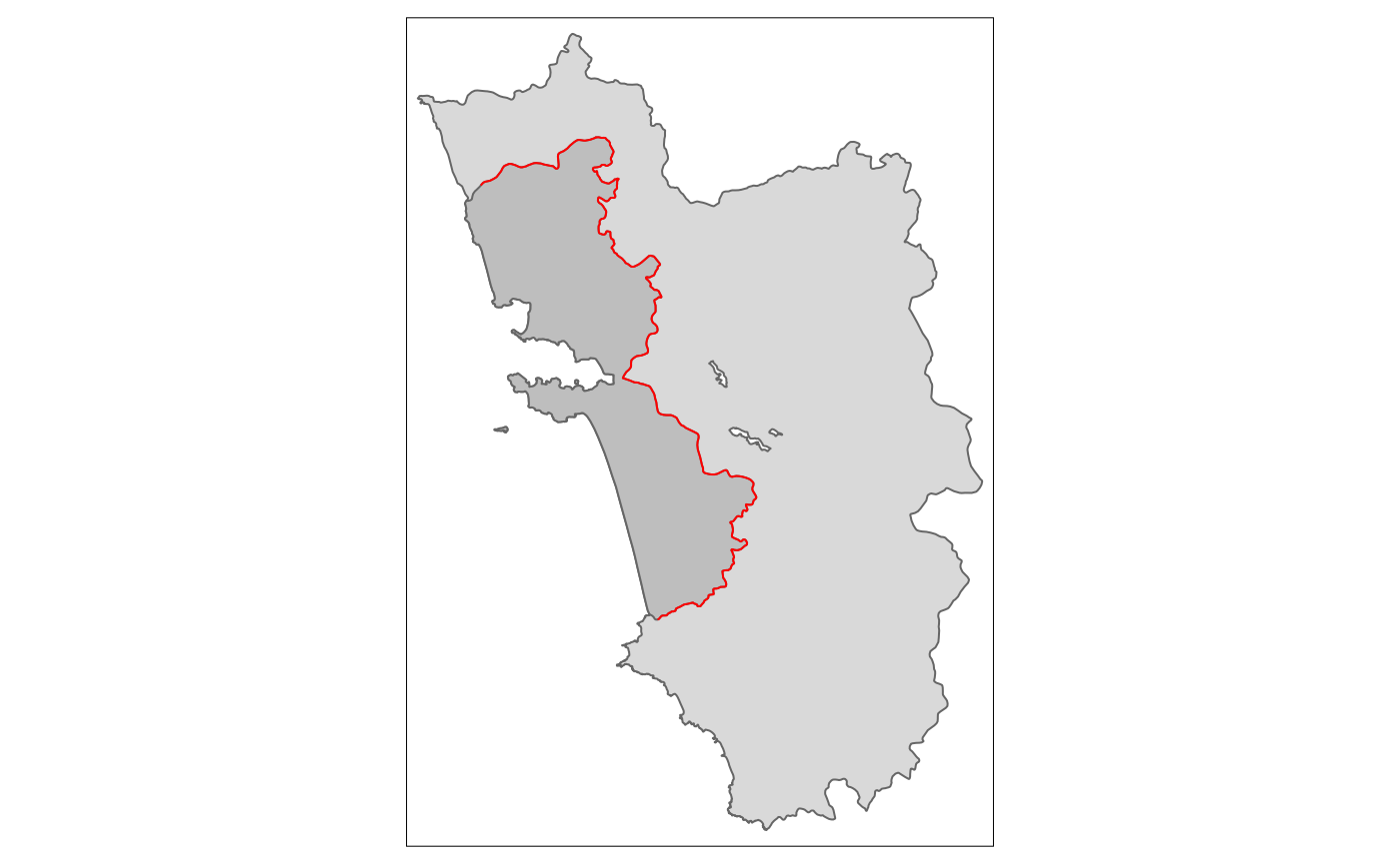

Above we see the simple map, visualizing the “treated polygon” in a darker grey, and the tmap syntax that produced it.

Let’s simulate some random points within the polygon that describes the entire study area:

set.seed(1088) # set a seed to make the results replicable
points_samp.sf <- sf::st_sample(polygon_full, 1000)
points_samp.sf <- sf::st_sf(points_samp.sf) # make it an sf object bc st_sample only created the geometry list-column (sfc)
points_samp.sf$id <- 1:nrow(points_samp.sf) # add a unique ID to each observation
# visualise results together with the line that represents our RDD cutoff
tm_shape(points_samp.sf) + tm_dots() + tm_shape(cut_off) + tm_lines(col = "red")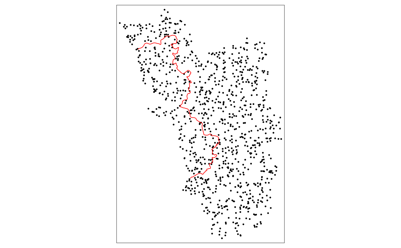

Assign Treatment

Now we use the first function of the SpatialRDD package. assign_treated() in essence just does a spatial intersection and returns a column vector that contains 0 or 1, depending on whether the observation is inside or outside the treatment area. Thus, we just add it as a new column to the points object. The function requires the name of the points object, the name of the polygon that defines the treated area, and the id that uniquely identifies each observation in the points object:

points_samp.sf$treated <- assign_treated(points_samp.sf, polygon_treated, id = "id")
tm_shape(points_samp.sf) + tm_dots("treated", palette = "Set1") + tm_shape(cut_off) + tm_lines(col = "red")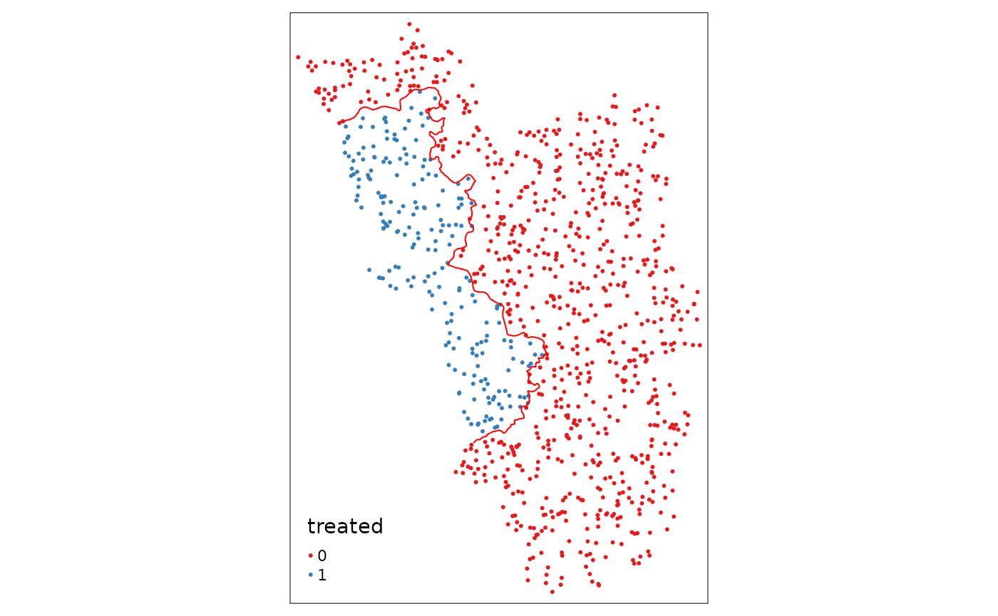

As a next step we add an outcome of interest that we are going to use as dependent variable in our Spatial Regression Discontinuity Design. Let’s call this variable education and assume it measures the literacy rate that ranges from 0 to 1 (0%, meaning everyone is illiterate, to 100%, meaning everyone in the population can read and write). We assume that the units, call them villages, in the “treated” polygon have on average a higher literacy rate because they received some sort of “treatment”. Let’s just assume someone magically dropped (better) schools in all of these villages, but not in any of the outside villages, and everything else is constant and identical across the two territories. Crucially, people also do not sort themselves across the border, i.e. they do not go on the other side to attend school and then return to their villages.

# first we define a variable for the number of "treated" and control which makes the code more readable in the future
NTr <- length(points_samp.sf$id[points_samp.sf$treated == 1])
NCo <- length(points_samp.sf$id[points_samp.sf$treated == 0])
# the treated areas get a 10 percentage point higher literacy rate
points_samp.sf$education[points_samp.sf$treated == 1] <- 0.7
points_samp.sf$education[points_samp.sf$treated == 0] <- 0.6
# and we add some noise, otherwise we would obtain regression coeffictions with no standard errors
# we draw from a normal with mean 0 and a standard devation of 0.1
points_samp.sf$education[points_samp.sf$treated == 1] <- rnorm(NTr, mean = 0, sd = .1) +
  points_samp.sf$education[points_samp.sf$treated == 1]
points_samp.sf$education[points_samp.sf$treated == 0] <- rnorm(NCo, mean = 0, sd = .1) +
  points_samp.sf$education[points_samp.sf$treated == 0]

# let's also add a placebo outcome that has no jump
points_samp.sf$placebo <- rnorm(nrow(points_samp.sf), mean = 1, sd = .25)

# visualisation split up by groups
library(ggplot2)
ggplot(points_samp.sf, aes(x = education)) + geom_histogram(binwidth = .01) + facet_grid(treated ~ .)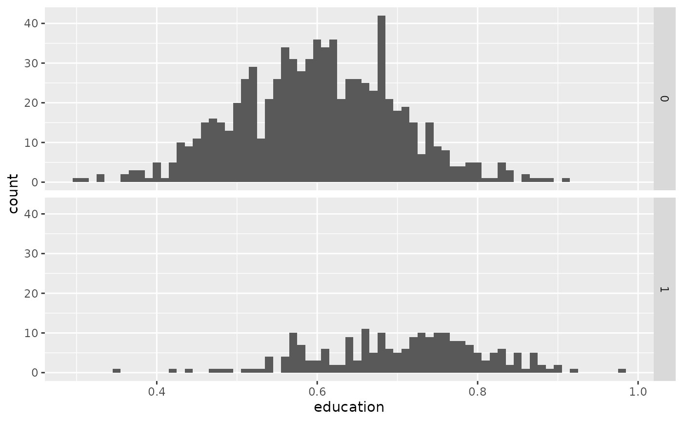

From the above histograms we can see that we were successful in creating different group means. This is also confirmed by the simple univariate regression of $y_i = \alpha + \beta\ \unicode{x1D7D9}(treated)_i + \varepsilon_i$:

list(lm(education ~ treated, data = points_samp.sf),
     lm(placebo   ~ treated, data = points_samp.sf)) %>% stargazer::stargazer(type = "text")
#> 
#> ===========================================================
#>                                    Dependent variable:     
#>                                ----------------------------
#>                                   education      placebo   
#>                                      (1)           (2)     
#> -----------------------------------------------------------
#> treated1                          0.100***        0.035*   
#>                                    (0.008)       (0.020)   
#>                                                            
#> Constant                          0.600***       0.990***  
#>                                    (0.004)       (0.009)   
#>                                                            
#> -----------------------------------------------------------
#> Observations                        1,000         1,000    
#> R2                                  0.160         0.003    
#> Adjusted R2                         0.160         0.002    
#> Residual Std. Error (df = 998)      0.100         0.260    
#> F Statistic (df = 1; 998)        186.000***       3.100*   
#> ===========================================================
#> Note:                           *p<0.1; **p<0.05; ***p<0.01

where the intercept tells us that the average in the non-treated areas is 0.6 and treated villages have on average a 10 percentage points higher education level.

Distance to Cutoff

The next essential step before we start to do proper spatial RDD analysis is to determine how far each of these points is away from the cutoff. Here we just make use of a function from sf called st_distance() that returns a vector with units (that we have to convert to real numbers by as.numeric()):

points_samp.sf$dist2cutoff <- as.numeric(sf::st_distance(points_samp.sf, cut_off))

This allows us now to investigate villages only within a specific range, say 3 kilometers, around our “discontinuity”:

tm_shape(points_samp.sf[points_samp.sf$dist2cutoff < 3000, ]) + tm_dots("education", palette = "RdYlGn", size = .1) + 
  tm_shape(cut_off) + tm_lines()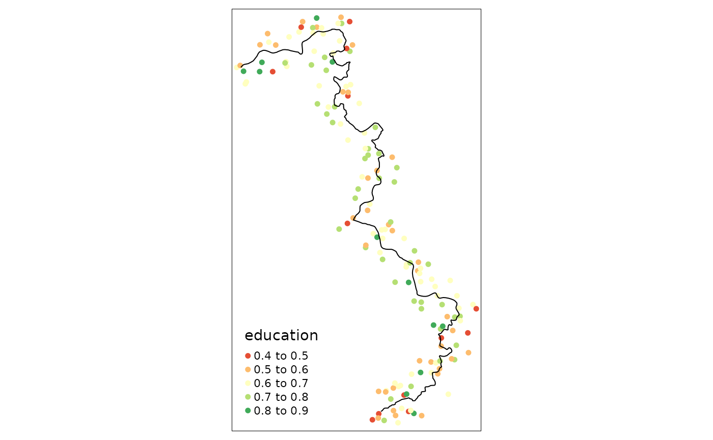

And to run the univariate regression from above also just within a bandwidth (this specification is already starting to resemble the canonical RD specification). As we know the exact data generating process (no “spatial gradient” but a rather uniform assignment), it is obvious to us that this of course leaves the point estimate essentially unchanged:

lm(education ~ treated, data = points_samp.sf[points_samp.sf$dist2cutoff < 3000, ]) %>% stargazer::stargazer(type = "text")
#> 
#> ===============================================
#>                         Dependent variable:    
#>                     ---------------------------
#>                              education         
#> -----------------------------------------------
#> treated1                     0.090***          
#>                               (0.015)          
#>                                                
#> Constant                     0.610***          
#>                               (0.011)          
#>                                                
#> -----------------------------------------------
#> Observations                    159            
#> R2                             0.190           
#> Adjusted R2                    0.180           
#> Residual Std. Error      0.095 (df = 157)      
#> F Statistic           36.000*** (df = 1; 157)  
#> ===============================================
#> Note:               *p<0.1; **p<0.05; ***p<0.01

Carrying out Spatial RDD estimation

Now we go step by step through all potential (parametric and non-parametric) ways in which one could obtain point estimates for Spatial RDDs (see e.g. Lehner2024? for details).

Unidimensional Specifications

Before we can run the RD, we need to transform the distance variable into a score. In this case, we can just multiply the distances on one side of the border with -1. To verify, let’s visualize the RDD by plotting all datapoints with the outcome on the y-axis and the score on the x-axis:

points_samp.sf$distrunning <- points_samp.sf$dist2cutoff
# give the non-treated one's a negative score
points_samp.sf$distrunning[points_samp.sf$treated == 0] <- -1 * points_samp.sf$distrunning[points_samp.sf$treated == 0]
ggplot(data = points_samp.sf, aes(x = distrunning, y = education)) + geom_point() + geom_vline(xintercept = 0, col = "red")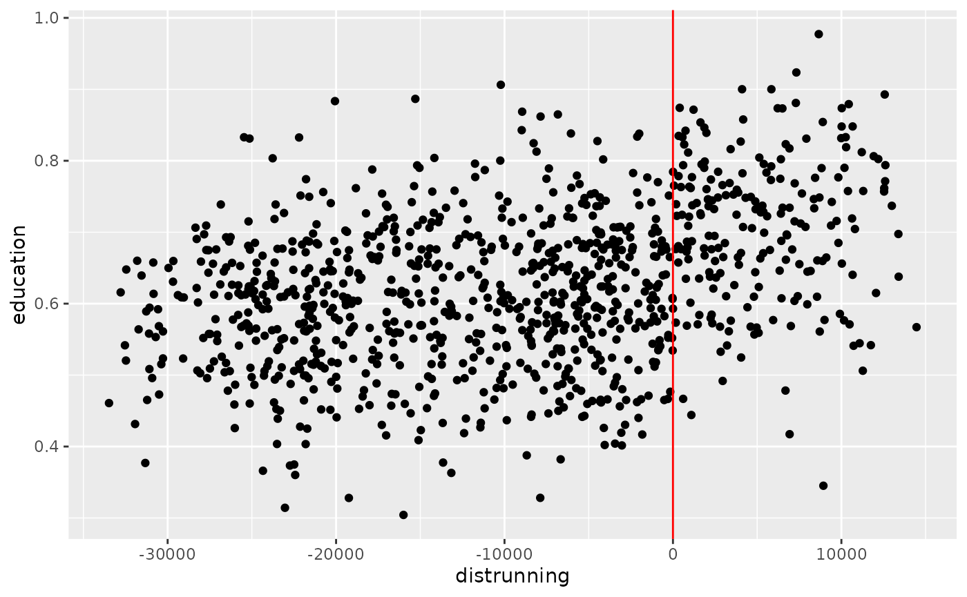

To obtain the point estimate, we use the fantastic rdrobust package (Calonico, Cattaneo, and Titiunik 2015). The default estimates an mserd bandwidth with a triangular kernel:

library(rdrobust)
rdbws <- rdrobust::rdbwselect(points_samp.sf$education, points_samp.sf$distrunning, kernel = "uniform") # save the bw
summary(rdrobust(points_samp.sf$education, points_samp.sf$distrunning, c = 0, kernel = "uniform"))
#> Sharp RD estimates using local polynomial regression.
#> 
#> Number of Obs.                 1000
#> BW type                       mserd
#> Kernel                      Uniform
#> VCE method                       NN
#> 
#> Number of Obs.                  785          215
#> Eff. Number of Obs.             113           90
#> Order est. (p)                    1            1
#> Order bias  (q)                   2            2
#> BW est. (h)                3806.072     3806.072
#> BW bias (b)                7347.289     7347.289
#> rho (h/b)                     0.518        0.518
#> Unique Obs.                     785          215
#> 
#> =============================================================================
#>         Method     Coef. Std. Err.         z     P>|z|      [ 95% C.I. ]       
#> =============================================================================
#>   Conventional     0.114     0.025     4.537     0.000     [0.065 , 0.163]     
#>         Robust         -         -     4.297     0.000     [0.066 , 0.177]     
#> =============================================================================

The according visualization with data driven bin-width selection and the local linear regression lines within the mserd bandwidth:

rdplot(points_samp.sf$education, points_samp.sf$distrunning, c = 0, ci = 95, p = 1,
       h = rdbws$bws[1],
       kernel = "triangular", y.label = "education", x.label = "distance to border")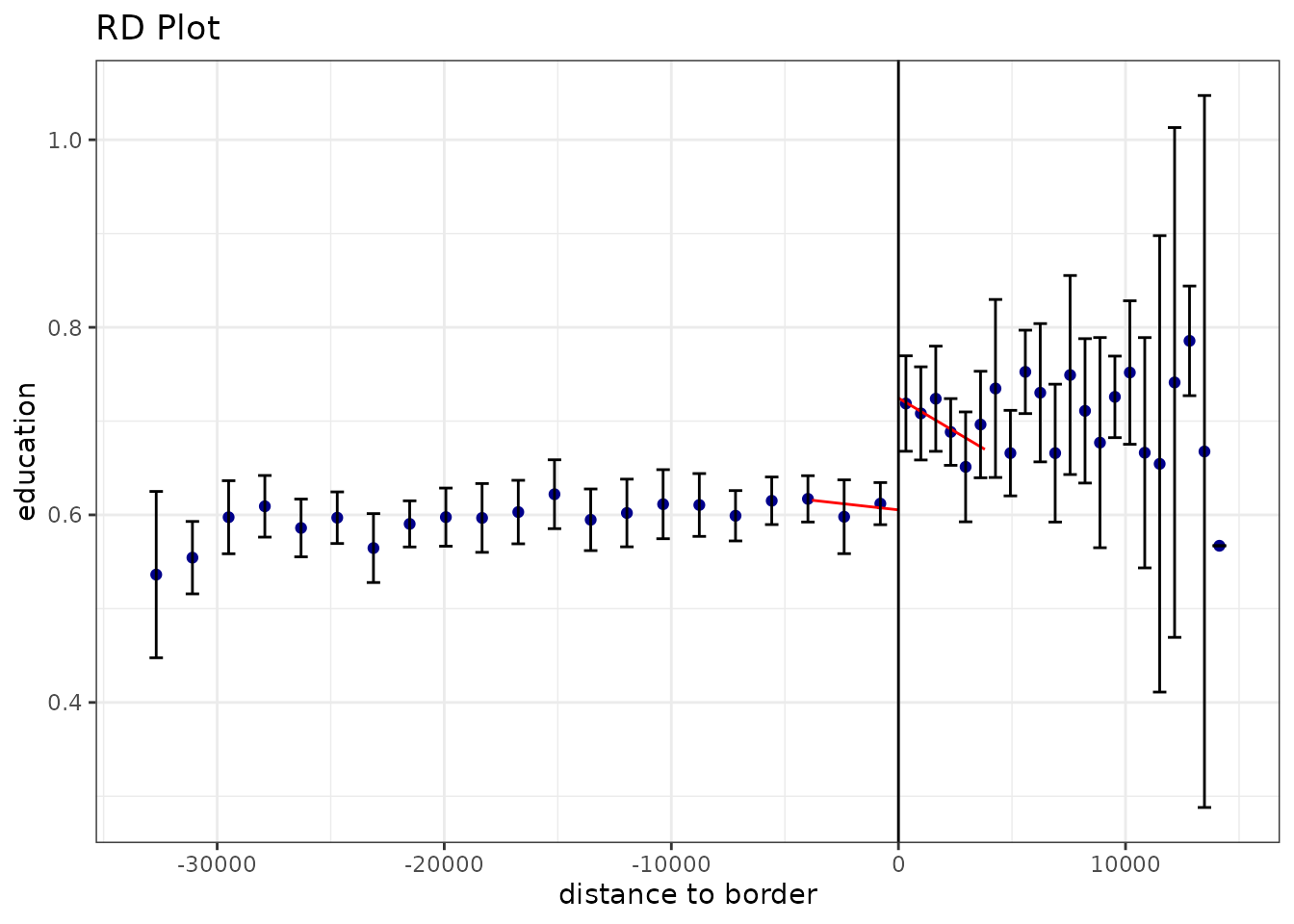

The same point estimate can be obtained through OLS by estimating

\[Y_i = \beta_0 + \beta_1\ D_i + \beta_2\ (X_i - c) + \beta_3\ D_i \times (X_i - c) + \varepsilon_i.\] This amounts to running:

list(lm(education ~ treated*distrunning, data = points_samp.sf[points_samp.sf$dist2cutoff < rdbws$bws[1], ])) %>% stargazer::stargazer(type = "text")
#> 
#> ================================================
#>                          Dependent variable:    
#>                      ---------------------------
#>                               education         
#> ------------------------------------------------
#> treated1                      0.110***          
#>                                (0.026)          
#>                                                 
#> distrunning                    0.00000          
#>                               (0.00001)         
#>                                                 
#> treated1:distrunning          -0.00002          
#>                               (0.00001)         
#>                                                 
#> Constant                      0.610***          
#>                                (0.017)          
#>                                                 
#> ------------------------------------------------
#> Observations                     203            
#> R2                              0.200           
#> Adjusted R2                     0.190           
#> Residual Std. Error       0.095 (df = 199)      
#> F Statistic            17.000*** (df = 3; 199)  
#> ================================================
#> Note:                *p<0.1; **p<0.05; ***p<0.01

… which is the same point estimate as above.

Adding Boundary Segment Fixed Effects

To ensure that only observations that are close to eachother are compared, we can create boundary segment categories. These are then used to apply a “within estimator” to allow for different intercepts for each of those segment categories. As is well known, instead of a within transformation, one might as well throw a set of dummies for each of the segments in the regression. The regression coefficient of interest of this saturated model then gives a weighted average over all segments. On top of that we might also be interested in the coefficient of each segment to infer something about potential heterogeneity alongside our regression discontinuity.
The (computationally a bit demanding) function border_segment() only needs the points layer and the cutoff as input (preferably as a line, but also an input in the form of points at the boundary works). The function’s last parameter lets us determine how many segments we want. As with the assign_treated() function, the output is a vector of factors.

points_samp.sf$segment10 <- border_segment(points_samp.sf, cut_off, 10)
points_samp.sf$segment15 <- border_segment(points_samp.sf, cut_off, 15)
tm_shape(points_samp.sf) + tm_dots("segment10", size = 0.1) + tm_shape(cut_off) + tm_lines()
tm_shape(points_samp.sf) + tm_dots("segment15", size = 0.1) + tm_shape(cut_off) + tm_lines()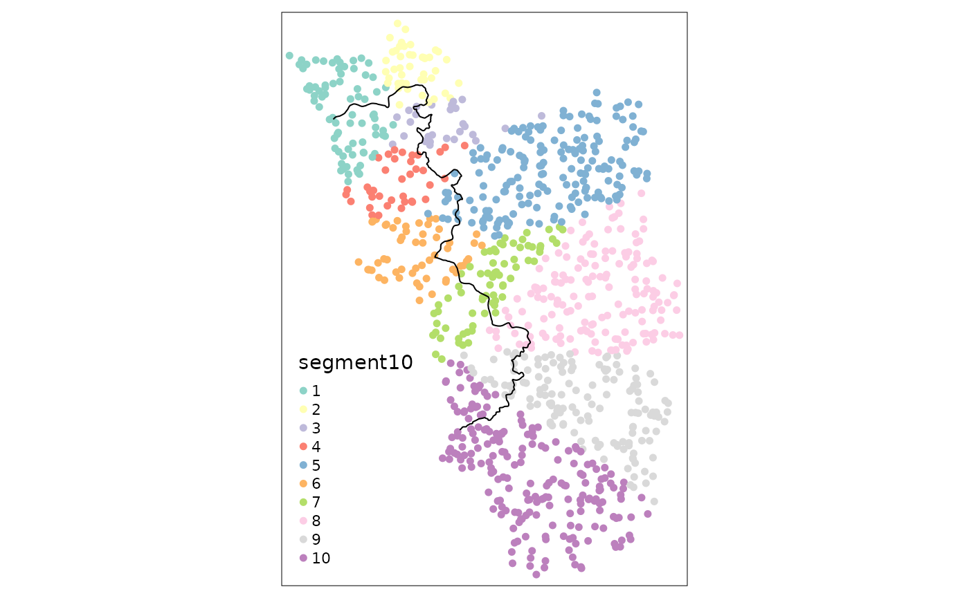

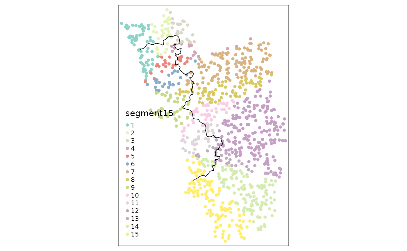
It is worth noting that the researcher has to pay attention to how the fixed effects are assigned. It could, e.g. due to odd bendings of the cutoff, be the case that for some segments only one side actually gets assigned a point. These situations are undesirable for two main reasons. First, estimation with segments that contain either only treated or only untreated units will be dropped automatically. Second, fixed effects category with a small amount of observations are not very informative for estimation. It is thus paramount to always plot the fixed effect categories on a map. The border_segment() already gives the researcher a feeling for how meaningful the choice for the number of segments was. In the above example we have a segment for every 13 kilometers, which seems not too unreasonable. We could already see however, that some of the categories contain very little observations. In the following example, we thus choose fewer border points, leading to more observations on each side of the border for every segment and thus to more meaningful point estimates:

points_samp.sf$segment5 <- border_segment(points_samp.sf, cut_off, 5)
tm_shape(points_samp.sf) + tm_dots("segment5", size = 0.1) + tm_shape(cut_off) + tm_lines()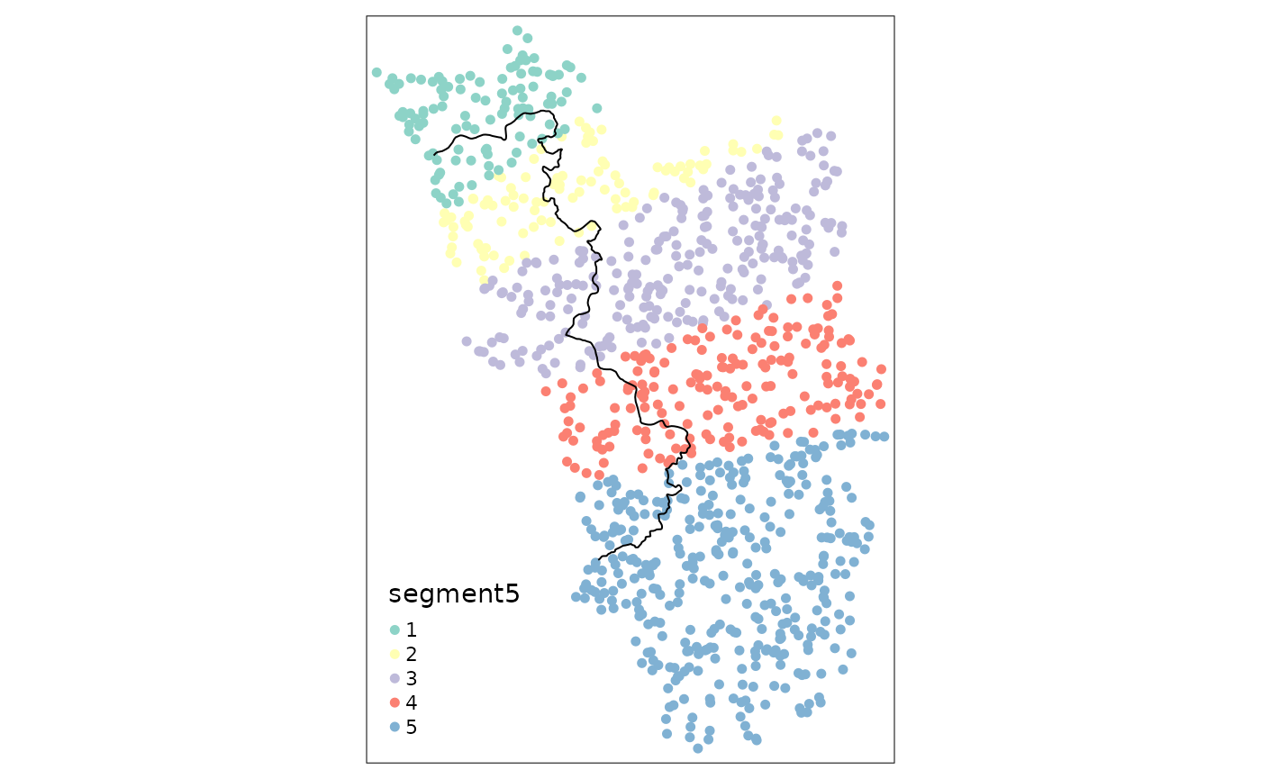

Simple OLS estimates, using the segments that we just obtained as categories for our fixed effects, show these differences:

library(lfe)
#> Loading required package: Matrix
list(lfe::felm(education ~ treated*distrunning | factor(segment15) | 0 | 0, data = points_samp.sf[points_samp.sf$dist2cutoff < rdbws$bws[1], ]),
lfe::felm(education ~ treated*distrunning | factor(segment5) | 0 | 0, data = points_samp.sf[points_samp.sf$dist2cutoff < rdbws$bws[1], ])
) %>% stargazer::stargazer(type = "text")
#> 
#> ======================================================
#>                             Dependent variable:       
#>                      ---------------------------------
#>                                  education            
#>                            (1)              (2)       
#> ------------------------------------------------------
#> treated1                 0.110***         0.110***    
#>                          (0.027)          (0.026)     
#>                                                       
#> distrunning              -0.00000         0.00000     
#>                         (0.00001)        (0.00001)    
#>                                                       
#> treated1:distrunning     -0.00001         -0.00002    
#>                         (0.00001)        (0.00001)    
#>                                                       
#> ------------------------------------------------------
#> Observations               203              203       
#> R2                        0.280            0.240      
#> Adjusted R2               0.210            0.220      
#> Residual Std. Error  0.094 (df = 185) 0.093 (df = 195)
#> ======================================================
#> Note:                      *p<0.1; **p<0.05; ***p<0.01

We obtain a point estimate that is (unsurprisingly, as we have a data generating process that is very uniform across space) essentially the same as the “classic RD” point estimate that we obtained from the non-parametric local linear regression from the rdrobust package (or the OLS equivalent with interaction) without segment fixed effects.

Specification With Two-Dimensional Score

Finally, we move towards a exploiting the two-dimensional nature of a spatial RDD. The function spatialrd() incorporates the RD estimation on any boundary point with just one line of code. This allows us to visualize the treatment effect at multiple points of the cutoff and thus infer something about the potential heterogeneity of the effect. Or, most importantly, to assess the robustness of the design itself.

First of all we have to cut the border into equally spaced segments. We will obtain a point estimate for each of these segments, or boundary points. The discretise_border() function just requires the sf object that represent the cutoff (polyline preferred but also points possible) and the number of desired boundary points:

borderpoints.sf <- discretise_border(cutoff = cut_off, n = 50)
borderpoints.sf$id <- 1:nrow(borderpoints.sf)
# exclude some of the borderpoints with little n so that the vignette can compile without warning:
#borderpoints.sf <- borderpoints.sf %>% slice(c(5,10,20,30,40))
tm_shape(points_samp.sf[points_samp.sf$dist2cutoff < 3000, ]) + tm_dots("education", palette = "RdYlGn", size = .1) +
  tm_shape(cut_off) + tm_lines() +
  tm_shape(borderpoints.sf) + tm_symbols(shape = 4, size = .3)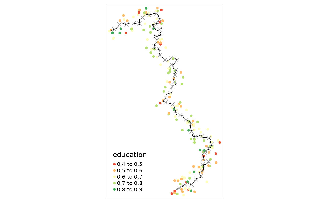

For plotting just a results table, it would be preferrable to choose just a data.frame as output (spatial.object = FALSE).

results <- spatialrd(y = "education", data = points_samp.sf, cutoff.points = borderpoints.sf, treated = "treated", minobs = 10, spatial.object = F)
knitr::kable(results)

Point	Estimate	SE_Conv	SE_Rob	p_Conv	p_Rob	Ntr	Nco	bw_l	bw_r	CI_Conv_l	CI_Conv_u	CI_Rob_l	CI_Rob_u
1	0.12	0.05	0.06	0.02	0.05	53	55	14.2	14.2	0.02	0.21	0.00	0.24
2	0.14	0.07	0.08	0.04	0.07	71	57	15.2	15.2	0.00	0.27	-0.01	0.30
3	0.11	0.05	0.06	0.02	0.06	103	84	19.9	19.9	0.02	0.21	0.00	0.24
4	0.08	0.05	0.06	0.11	0.22	100	65	16.0	16.0	-0.02	0.17	-0.05	0.20
5	0.08	0.05	0.06	0.11	0.22	104	73	17.3	17.3	-0.02	0.17	-0.04	0.19
6	0.07	0.04	0.05	0.09	0.22	112	84	20.9	20.9	-0.01	0.15	-0.04	0.16
7	0.06	0.03	0.04	0.08	0.20	108	62	18.9	18.9	-0.01	0.13	-0.03	0.13
8	0.07	0.04	0.05	0.10	0.18	93	46	17.1	17.1	-0.01	0.15	-0.03	0.16
9	0.11	0.07	0.08	0.09	0.11	77	33	14.1	14.1	-0.02	0.24	-0.03	0.27
10	0.13	0.07	0.08	0.04	0.05	69	32	12.3	12.3	0.01	0.26	0.00	0.30
11	0.18	0.07	0.08	0.01	0.02	56	32	11.1	11.1	0.04	0.32	0.03	0.35
12	0.25	0.12	0.13	0.03	0.03	40	22	9.6	9.6	0.02	0.48	0.02	0.53
13	0.32	0.14	0.15	0.02	0.02	29	17	8.2	8.2	0.04	0.60	0.05	0.65
14	0.20	0.07	0.08	0.01	0.01	33	32	9.5	9.5	0.06	0.35	0.06	0.40
15	0.15	0.06	0.07	0.01	0.01	24	30	8.8	8.8	0.03	0.27	0.04	0.32
16	0.16	0.05	0.06	0.00	0.00	52	86	13.7	13.7	0.06	0.25	0.06	0.28
17	0.18	0.06	0.07	0.00	0.00	30	45	10.7	10.7	0.07	0.29	0.07	0.33
18	0.15	0.06	0.07	0.01	0.02	56	98	14.5	14.5	0.04	0.26	0.02	0.29
19	0.11	0.05	0.06	0.02	0.09	96	102	16.4	16.4	0.01	0.20	-0.01	0.21
20	0.10	0.06	0.07	0.08	0.16	85	56	13.9	13.9	-0.01	0.21	-0.04	0.23
21	0.08	0.05	0.06	0.11	0.22	80	39	13.2	13.2	-0.02	0.19	-0.05	0.20
22	0.07	0.06	0.07	0.21	0.35	73	53	13.3	13.3	-0.04	0.19	-0.07	0.20
23	0.10	0.05	0.06	0.04	0.12	96	52	14.1	14.1	0.00	0.20	-0.02	0.21
24	0.10	0.05	0.07	0.05	0.14	103	60	14.5	14.5	0.00	0.21	-0.03	0.23
25	0.10	0.06	0.07	0.10	0.23	83	57	13.6	13.6	-0.02	0.22	-0.06	0.24
26	0.06	0.07	0.09	0.43	0.64	55	49	11.7	11.7	-0.09	0.20	-0.13	0.22
27	0.05	0.08	0.10	0.56	0.80	37	38	9.6	9.6	-0.11	0.21	-0.17	0.22
30	0.01	0.09	0.11	0.88	0.95	32	34	9.2	9.2	-0.17	0.19	-0.22	0.21
31	0.08	0.06	0.07	0.20	0.35	65	61	12.8	12.8	-0.04	0.19	-0.08	0.21
32	0.11	0.06	0.07	0.07	0.14	47	39	10.6	10.6	-0.01	0.22	-0.03	0.24
33	0.10	0.04	0.05	0.01	0.04	102	68	14.9	14.9	0.02	0.17	0.00	0.20
34	0.10	0.04	0.05	0.01	0.02	109	63	14.8	14.8	0.03	0.18	0.02	0.20
35	0.11	0.04	0.05	0.01	0.02	53	47	11.3	11.3	0.02	0.19	0.02	0.22
36	0.17	0.03	0.03	0.00	0.00	24	25	8.6	8.6	0.11	0.23	0.12	0.25
37	0.15	0.05	0.06	0.00	0.01	38	21	8.6	8.6	0.05	0.26	0.05	0.29
38	0.15	0.06	0.07	0.01	0.02	108	44	13.4	13.4	0.04	0.25	0.02	0.29
39	0.13	0.05	0.06	0.01	0.02	167	64	16.5	16.5	0.03	0.22	0.03	0.26
40	0.14	0.05	0.06	0.01	0.01	137	62	15.1	15.1	0.04	0.24	0.04	0.28
41	0.18	0.06	0.07	0.00	0.00	61	45	11.1	11.1	0.06	0.30	0.07	0.34
42	0.15	0.06	0.07	0.01	0.01	57	50	10.9	10.9	0.03	0.26	0.04	0.30
43	0.13	0.05	0.06	0.01	0.01	152	64	15.5	15.5	0.04	0.22	0.04	0.25
44	0.11	0.06	0.07	0.04	0.05	99	60	13.3	13.3	0.01	0.22	0.00	0.26
45	0.10	0.05	0.06	0.04	0.05	111	59	13.8	13.8	0.01	0.20	0.00	0.23
46	0.11	0.06	0.08	0.09	0.10	112	52	13.4	13.4	-0.02	0.23	-0.02	0.28
47	0.08	0.05	0.06	0.12	0.13	130	60	15.5	15.5	-0.02	0.18	-0.03	0.21
48	0.06	0.04	0.05	0.12	0.18	233	75	23.0	23.0	-0.02	0.15	-0.03	0.18
49	0.06	0.04	0.06	0.17	0.23	162	67	19.6	19.6	-0.03	0.15	-0.04	0.17
50	0.05	0.04	0.05	0.24	0.35	112	60	17.6	17.6	-0.03	0.12	-0.05	0.14

The average treatment effect is given by taking the mean of all point estimates because there is no heterogeneity. Otherwise it would be necessary to weigh the point estimate at each boundary point (by the respective sample size, for example). Running mean(results$Estimate) this gives 0.12, which is exactly how we designed our DGP. For the plotting of boundarypoints and a visualization in space of each point estimate we need to have a spatial object. All this is incorporated in the plotspatialrd() function.

results <- spatialrd(y = "education", data = points_samp.sf, cutoff.points = borderpoints.sf, treated = "treated", minobs = 10)
plotspatialrd(results, map = T)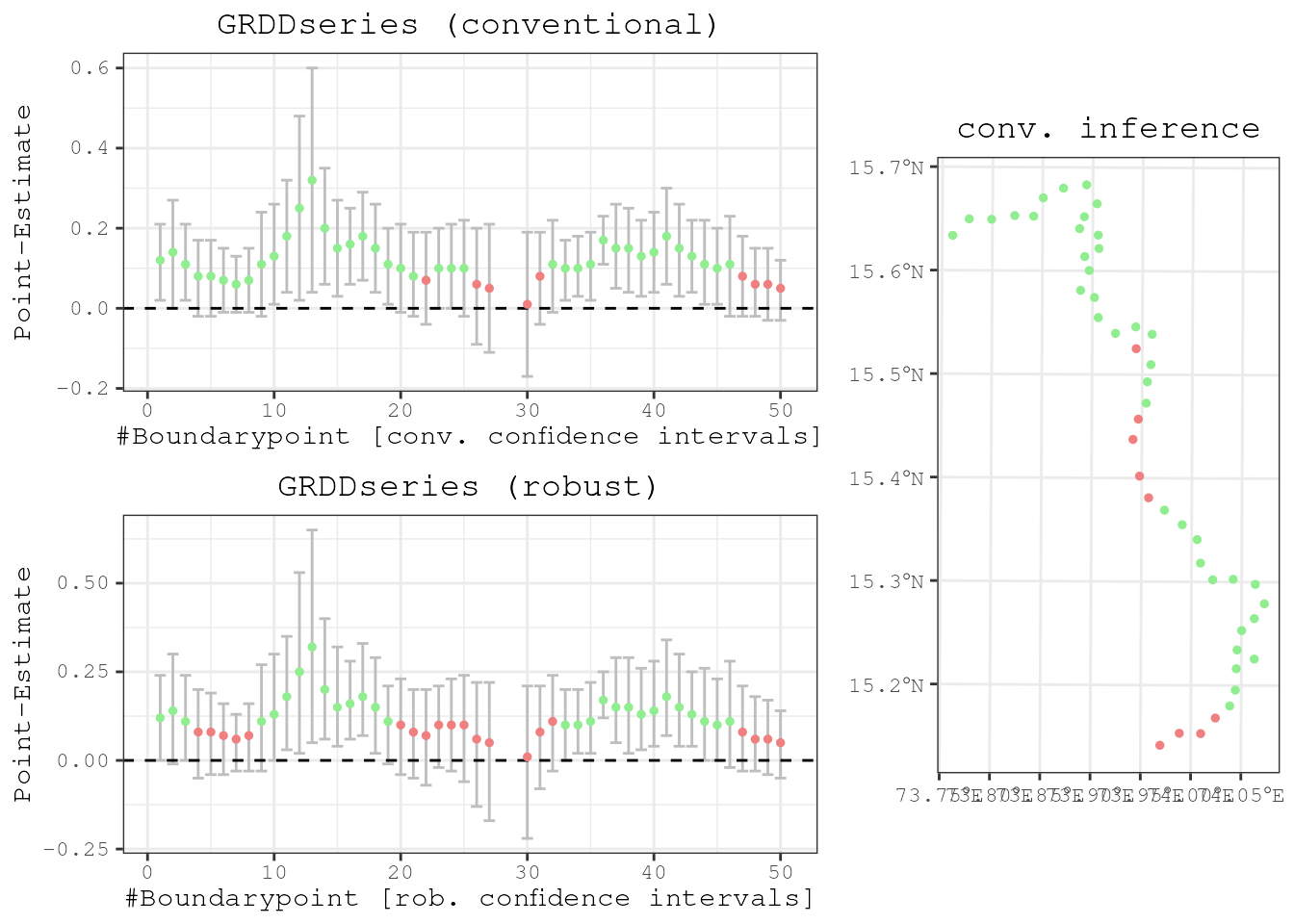

Or just the series of boundarypoints without the map.

plotspatialrd(results, map = F)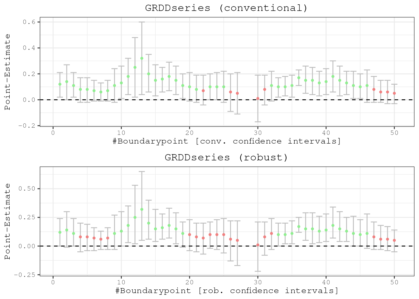

Robustness

In Spatial Regression Discontinuity exercises, the researcher usually also has to show that the results are robust towards different specifications and parameters. Also in this respect the SpatialRDD package offers a lot of capabilities that are time saving and make replicability easy. This toolbox for shifting and moving around borders and afterwards assigning (placebo) treatment status again is in fact so potent, that it is of use in many other research design settings outside of geographic RDs. In this vignette we will just see the basic intuition. For more details on all the options check out the separate vignette shifting_borders or go to the copy of the article on the package website.

Placebo Borders

Here we are going to apply a standard tool that we got to know in linear algebra 1 classes: an affine transformation of the type $f(x) = x\mathbf{A}+b$, where the matrix $\mathbf{A}$ is the projection matrix to shift, (re-)scale, or rotate the border. For simplicity we now only apply a shift by 3000 meters in both the x- and y-coordinates of the border.

placebocut_off.1 <- shift_border(cut_off, operation = "shift", shift = c(3000, 3000))
placeboborderpoints.1 <- discretise_border(cutoff = placebocut_off.1, n = 50)
tm_shape(points_samp.sf) + tm_dots("treated", palette = "Set1")  + tm_shape(placeboborderpoints.1) + tm_symbols(shape = 4, size = .3) + tm_shape(placebocut_off.1) + tm_lines()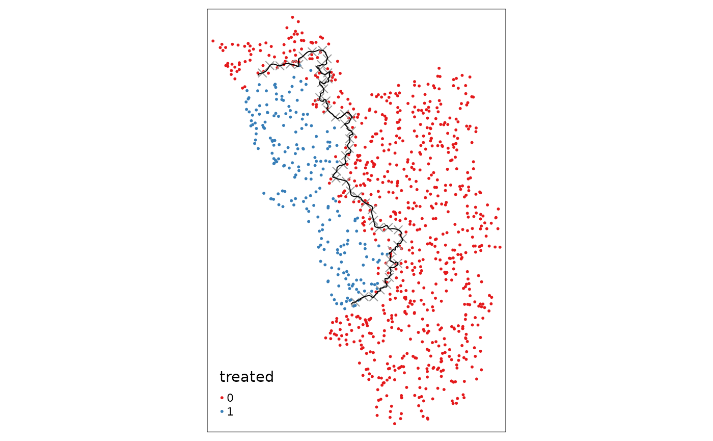

After the border shift we now have to re-assign the new treatment status in order to carry out regressions. For that matter, we create new polygons from scratch with the cutoff2polygons() function. The logic of this function is not very intuitive at first, but the vignette on border shifting will clarify that. In our case, we do not have to go around corners with the counterfactual polygon because both ends of the cutoff go towards the West. Just make sure that the endpoints are chosen in a way so that all observations that should be in the “placebo treated” group are also actually inside this resulting polygon.

placebo.poly.1 <- cutoff2polygon(data = points_samp.sf, cutoff = placebocut_off.1, orientation = c("west", "west"), endpoints = c(.8, .2))

tm_shape(placebo.poly.1) + tm_polygons(alpha = .3)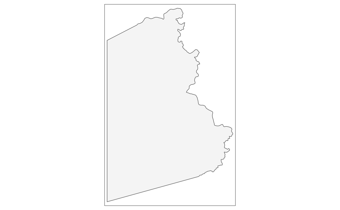

Finally, we have to use the assign_treated() function from the beginning of the vignette again:

points_samp.sf$treated1 <- assign_treated(data = points_samp.sf, polygon = placebo.poly.1, id = "id")
sum(points_samp.sf$treated == 0 & points_samp.sf$treated1 == 1) # number of villages that switched treatment status
#> [1] 60
tm_shape(points_samp.sf) + tm_dots("treated1", palette = "Set1")  + tm_shape(placeboborderpoints.1) + tm_symbols(shape = 4, size = .3) + tm_shape(placebocut_off.1) + tm_lines()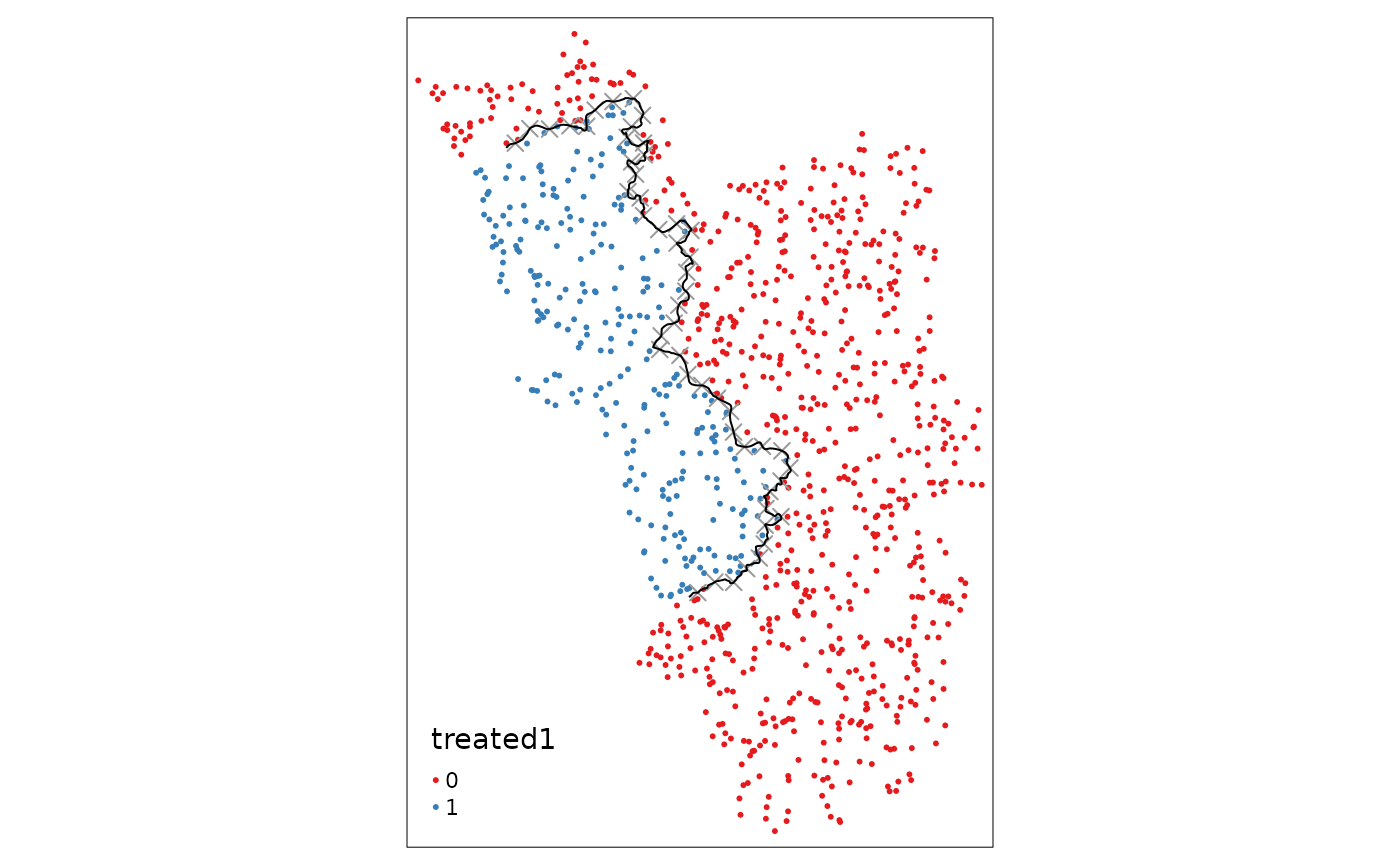

After plotting the points again, we can visually infer that the villages to the right got assigned the “treated” dummy. Further we can compute the number of villages that change their status. This helps us to decide whether the bordershift was big enough (if e.g. only a handful of observations switched, then we would expect this to have little to no impact on our point estimates and thus would dub such a robustness exercise as not very meaningful).
In this case 60 villages changed. Given the initial number of treated observations, this seems a change of a big enough magnitude and thus a meaningful robustness exercise.

Robustness With Two-Dimensional Score

Finally, we do the exact same exercise from above again and run the uni-dimensional RD specification on many boundary points to approximate a continuous treatment effect. The series fluctuates around 0 and has not a single significant estimate, and it is thus safe to conclude that the methodology works.

results1 <- spatialrd(y = "education", data = points_samp.sf, cutoff.points = placeboborderpoints.1, treated = "treated1", minobs = 10)
plotspatialrd(results1, map = T)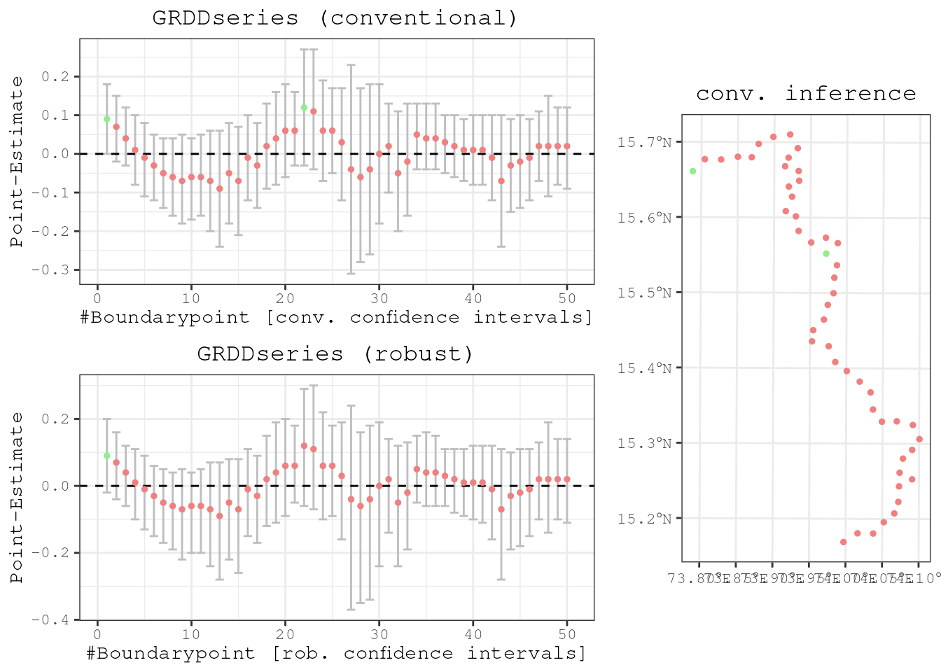

Robustness With Uni-Dimensional Specification

Before we close, let’s also run our placebo exercise with the uni-dimensional specification.

points_samp.sf$segment.1.5 <- border_segment(points_samp.sf, placebocut_off.1, 5) # assigning new segments based on now cutoff
points_samp.sf$dist2cutoff1 <- as.numeric(sf::st_distance(points_samp.sf, placebocut_off.1)) # recompute distance to new placebo cutoff

list(
  lm(education ~ treated1*distrunning, data = points_samp.sf[points_samp.sf$dist2cutoff1 < 3000, ])#,
  #lfe::felm(education ~ treated1*distrunning | factor(segment.1.5) | 0 | 0, data = points_samp.sf[points_samp.sf$dist2cutoff1 < 3000, ])
) %>% stargazer::stargazer(type = "text")
#> 
#> =================================================
#>                           Dependent variable:    
#>                       ---------------------------
#>                                education         
#> -------------------------------------------------
#> treated11                       -0.034           
#>                                 (0.026)          
#>                                                  
#> distrunning                   0.00002***         
#>                                (0.00001)         
#>                                                  
#> treated11:distrunning          -0.00000          
#>                                (0.00001)         
#>                                                  
#> Constant                       0.680***          
#>                                 (0.024)          
#>                                                  
#> -------------------------------------------------
#> Observations                      177            
#> R2                               0.089           
#> Adjusted R2                      0.073           
#> Residual Std. Error        0.096 (df = 173)      
#> F Statistic             5.600*** (df = 3; 173)   
#> =================================================
#> Note:                 *p<0.1; **p<0.05; ***p<0.01

References

Bivand, Roger, and Edzer Pebesma. 2023. Spatial Data Science: With Applications in r. New York: Chapman; Hall/CRC. https://doi.org/10.1201/9780429459016.

Calonico, Sebastian, Matias D. Cattaneo, and Rocío Titiunik. 2015. “Rdrobust: An r Package for Robust Nonparametric Inference in Regression-Discontinuity Designs.” R Journal 7 (1): 38–51.

Lehner, Alexander. 2023. “Culture, Institutions, and the Roots of Gender Inequality: 450 Years of Portuguese Colonialism in India.” Mimeograph.

Alexander Lehner

2024-03-21